Beginner's Guide to Principal Components
by Kilem Li Gwet, PhD
Principal Component Analysis (PCA) is a statistical technique (not a machine learning algorithm) widely used today for dimensionality reduction of a large dataset. It is believed to have been invented in 1901 and has been used by statisticians and social scientits for more than 100 years. However, the interest in PCA has dramatically increased in the era of big data and many modern data processing systems used a version of it.
How exactly does PCA reduce dimensionality? What price do we pay for reducing dimensionality? Look at Figure 1. It shows a scatterplot of original data points in red color. Any exploratory analysis of that data requires that we look at both the $x$ and the $y$ dimensions. Therefore, we are dealing with a 2-dimensional problem where each data point is represented by 2 coordinates $(x,y)$ on the standard coordinate system defined by the 2 basis vectors $(\vec{\imath},\vec{\jmath})$.
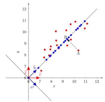
Figure 1: Orthogonal projection onto the first principal component
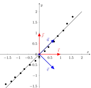
Figure 2: Almost perfect representation of data points on the first principal component
Here is a fundamental fact all beginners must understand about PCA:
There is no requirement whatsoever to use the standard coordinate system that the 2 basis vectors $(\vec{\imath},\vec{\jmath})$ define. As a matter of fact, any 2 orthogonal vectors can define a new and valid coordinate system. It turned out that some special orthogonal vectors define coordinate systems that are convenient for analysis.Consider for example the 2 orthogonal vectors $(\vec{u},\vec{v})$ in Figure 1. Vector $\vec{u}$ defines the dimension along which the data points vary the most, while vector $\vec{v}$ defines the dimension along which the data vary the least. If you want to analyze your data on a single dimension, it is certainly the dimension defined by vector $\vec{u}$ that you will want to retain. The data points in blue color are the orthogonal projections of the original red data points onto the axis defined by vector $\vec{u}$, and represent the numbers you will analyzed in the reduced one-dimensional space. Vector $\vec{u}$ is called the first (and most dominant) principal component, while vector $\vec{v}$ is the second and least dominant principal components.
The study of Principal Components amounts to doing the following:
- Determine mathematically the 2 coordinates of the 2 principal components $\vec{u}$ and $\vec{v}$ in the standard coordinate system. In fact, these are 2 eigenvectors of the correlation matrix associated with the 2 variables $x$ and $y$.
- Find what the coordinates of the original data points are on the new coordinate system of principal components. These are called the Principal Component Scores. That is, there is expected to be one series of principal component scores associated with $\vec{u}$ and a second series of principal component scores associated with $\vec{v}$. The eigenvalue $\lambda_u$ associated with vector $\vec{u}$ is also the variance of the related series of principal component scores. The same can be said about the eigenvalue $\lambda_v$ and its associated vector $\vec{v}$.
- Interpret the principal components with respect to the original variables. This task is accomplished by calculating the pairwise covariances between each series of principal component scores and all original variables. These covariances are known as the principal component loadings.
All three tasks defined above and more are discussed in details in my book entitled Beginner's Guide to Principal Components. You may download the first few pages of each chapters for information below. Errors and typos contained in this book as reported by various readers and myself can be found in the errata page. Please check there regularly for new reports.
Contents
- Preliminaries: Preliminaries include the preface, the table of contents and the acknowledgement page.
- Chapter 1: Principal Components and Linear Algebra
- Chapter 2: Computing Principal Components
- Chapter 3: Using Principal Components
- Appendix A: Matrix Operations with Excel
- Appendix B: Matrices, Vectors and Calculus
- Appendix C: Miscellaneous Data Used in this Book
Beginner's Guide to Principal Components by Kilem L. Gwet, PhD
![]()